
Thursday, November 16, 2023
Correlation
Often, a primary goal of data analysis is to show the relationship between two variables. For example, how does the price of an apartment relate to its size? Does its distance from downtown affect the value as well? What about the year of construction or the level of noise in the neighborhood? Scatterplots help us answer such questions by giving us a visual representation of these relationships.
The tendency for one variable to change in relation to the change in another variable is called correlation.
The scatterplots we made in the last lesson show that height and weight are positively correlated. This makes sense because an increase in one generally means an increase in the other. An example of a negative correlation would be height and voice pitch; generally, the taller you are the lower the frequency of your voice.
Correlation coefficient
It’s one thing to look at a scatter plot, but we also need a numerical way to describe correlation.
For this we have the Pearson correlation coefficient, commonly just referred to as the correlation coefficient. It quantifies how one variable tends to change when the other variable changes. The correlation coefficient can take any value between -1 and 1, where -1 represents perfect linear negative correlation and 1 represents perfect linear positive correlation. Generally, it works like this:
- If one value increases together with the other, the correlation coefficient is positive
- If one remains the same when the other changes, the coefficient is 0
- If one decreases when the other increases, the coefficient is negative
The closer the coefficient is to -1 or 1, the stronger the correlation. On the other hand, a value of 0 can mean either that there’s no correlation or that there’s a complex non-linear connection that the coefficient can’t reflect.
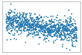
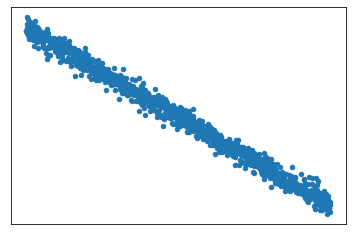
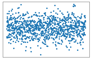
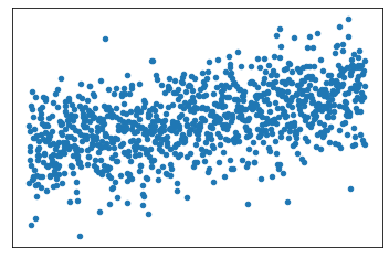
To help you get a sense of the relationship between the correlation coefficient and the distribution of points in a scatterplot, we’ve included an interactive figure where you can change the correlation coefficient to see how the spread of data points changes.
Note that there are many different scatterplots that could all result in the same correlation coefficient; this is just meant to be one example.
Quiz (matching)
Description
Match each scatterplot to the correlation coefficient that best describes its correlation:
Bins
Questions
A) 0.99
B) 0.5
C) 0
D) -0.5
E) -0.99

Calculating the correlation coefficient
In pandas, the Pearson correlation coefficient is calculated with the corr() method. It’s applied to the column containing the first variable, and the column with the second is passed as a parameter. It doesn’t matter which is which. For example:
import pandas as pd
from matplotlib import pyplot as plt

df = pd.read_csv('/datasets/height_weight.csv')

print(df['height'].corr(df['weight']))
0.9165261045538688
With a coefficient of about 0.9, height and weight have a strong positive correlation in this dataset. This matches with our “common sense” that taller people tend to weigh more. Of course, there is variation in this trend, so we wouldn’t expect a perfect positive correlation coefficient of 1.
It may be tempting to make a statement such as “a person’s height determines their weight”. But on its own, correlation can’t tell us anything about cause and effect; we only know that the two factors are correlated. To prove (or disprove) cause and effect, we would need to perform controlled experiments.
For now, let’s practice calculating correlation coefficients for other pairs of variables in our dataset.
Tasks
Task 1
Remember the scatterplot you made in the last lesson for the 'height' and 'age' columns? Calculate the Pearson correlation coefficient for those columns and assign the result to a variable called ah_corr. Then print it. Does the result align with the scatterplot?
Hint
Call corr() on either the 'height' or 'age' column of df and pass the other column as an argument. Assign the result to ah_corr, then use print() to display it.
Success text
Almost 0 correlation! That jives with the scatterplot. It also makes intuitive sense. The youngest age in this dataset is 25 years old. Most people are done growing by then.
Precode
import pandas as pd

df = pd.read_csv('/datasets/height_weight.csv')

# write your code here
Solution
import pandas as pd

df = pd.read_csv('/datasets/height_weight.csv')

ah_corr = df['height'].corr(df['age'])
print(ah_corr)
Output
0.010042046516844351
Task 2
Try calling the corr() method on the whole DataFrame. What happens? Print the result.
Hint
Call corr() on df and wrap it in a print() function.
Success text
It looks like pandas returned a DataFrame with the correlation coefficients for each pair of variables. Cool! Let’s learn more about that in the next lesson.
Precode
import pandas as pd

df = pd.read_csv('/datasets/height_weight.csv')

# write your code here
Solution
import pandas as pd

df = pd.read_csv('/datasets/height_weight.csv')

print(df.corr())
Output
          height    weight       age      male
height  1.000000  0.916526  0.010042  0.760690
weight  0.916526  1.000000  0.228538  0.785218
age     0.010042  0.228538  1.000000  0.004750
male    0.760690  0.785218  0.004750  1.000000